Kolmogorov-Arnold Networks (KAN)

Kolmogorov-Arnold Networks (KANs), introduced by Liu et al. in April 2024, rearrange where a neural network learns its transformations. A standard multilayer perceptron learns one scalar weight per edge and uses fixed activation functions at nodes. A KAN places a learned one-dimensional function on every edge; its nodes simply add incoming values.

What Lives on an Edge?

Switch architectures, then move the same input through one connection. The location of the learnable nonlinearity is the central difference.

Input x0.45

Edge computation

phi(x) = 0.696

x = 0.45

→

0.696

The entire curve is learned from spline coefficients.

A KAN edge stores a learned one-dimensional function. The receiving node only adds incoming values.

The inspiration is the Kolmogorov-Arnold representation theorem: a continuous multivariate function on a bounded domain can be represented using continuous univariate functions and addition. One channel has the form

$f\left(\phi_1(x_1)+\phi_2(x_2)+\cdots+\phi_n(x_n)\right).$

The classical representation adds several such outer-function channels. Modern KANs generalize the construction to arbitrary widths and depths by stacking KAN layers.

Trace One KAN Channel

Each input travels through its own univariate edge function. A node sums the transformed values; an outer edge function can then transform that sum.

Input x10.55Input x2-0.35Input x30.20

Outer function f

x1 = 0.55

phi1(x1)

0.648

x2 = -0.35

phi2(x2)

0.192

x3 = 0.20

phi3(x3)

0.295

sum = 1.135

→

f(s) = tanh(s)

→

y = 0.813

Selected outer transformation

f(1.135) = tanh(1.135)

y = 0.813

y = f(phi1(x1) + phi2(x2) + phi3(x3))

The classical representation sums several channels like this. A deep KAN generalizes the idea by composing whole KAN layers.

KAN edge functions are commonly parameterized with B-splines: smooth piecewise-polynomial curves built from overlapping basis functions. Their most useful property here is local control. Changing one coefficient reshapes a neighborhood of the curve while leaving distant regions alone.

B-Spline Edge Function in a KAN

A KAN edge learns a univariate function phi(x) from overlapping B-spline basis pieces. Drag knots along the curve to reposition them, or click the curve to add one.

This edge stays quiet for low inputs, then contributes strongly once x1 enters a sensitive range.

Interior knots (2)

knot 1 — 35%

knot 2 — 60%

Drag handles on the curve, or click the curve to add a knot (max 6).

Show individual basis functions

KAN edge function

phi(x) =+++++

Enable "Show basis functions" to highlight individual terms.

Composite edge function phi(x) Knot (drag to move)

The spline coefficients are trainable parameters of this KAN edge. Knot placement controls where the edge function has flexibility; adding more knots increases local detail but can also make the learned function harder to regularize and interpret.

Training still uses the familiar differentiable-learning loop. The parameters being updated are the coefficients that shape each edge function.

Train One Edge Function

Walk through one optimization loop. The visualization is simplified, but the update target is real: spline coefficients receive gradients through backpropagation.

Step 1

Initialize splines

Give every edge a spline grid and initial coefficients. At this point the curves do not yet match the data.

Epoch

0.0 / 8

Loss

0.4260

Curve fit

learned splinetarget function

KAN training uses the familiar differentiable-learning loop. What changes is the parameterization: optimization shapes functions on edges rather than only scalar weights.

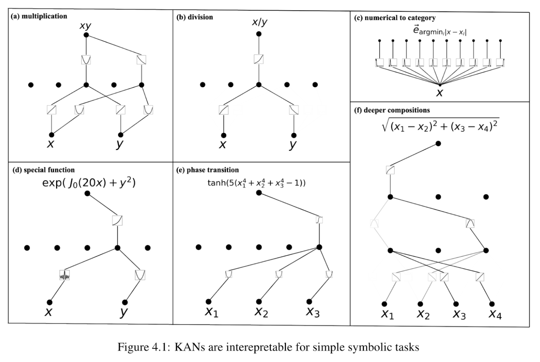
Because individual edge functions can be plotted, a trained KAN can support an interactive form of symbolic regression. The original workflow trains for sparsity, prunes weak structure, replaces promising spline shapes with candidate symbolic functions, and fine-tunes the resulting parameters.

From Splines to a Symbolic Formula

Move through the simplification workflow. Increase regularization to fade weak connections, then inspect what remains after pruning and symbolification.

Sparsity regularizationlambda = 0.35

Magnitude removed

16%

Illustrative fit loss

0.0119

Sparsify

Penalize the average magnitude of edge functions. Entropy regularization can help concentrate importance on fewer edges.

edge A0.94 → 0.90

learned spline

edge B0.08 → 0.02

candidate for pruning

edge C0.72 → 0.56

learned spline

edge D0.03 → 0.01

candidate for pruning

Nonzero edges

3 / 4

Current model

objective = prediction loss + 0.35 * sparsity penalty

A readable formula is a hypothesis to validate, not proof that the recovered expression is uniquely correct or causal.

◆

What symbolification fits

If a surviving edge resembles a known function $f$ , the exact spline may still be shifted and scaled. KAN tooling fits affine parameters so that $y \approx c f(ax+b)+d$ . The candidate function supplies the shape; $(a,b,c,d)$ align it with the observed pre- and post-activations.

⚠

Interpretability scales with size

Plottable edges do not make every KAN easy to understand. A wide, deep model can contain many composed functions, and symbolic matches may be unstable or non-unique. Evaluate readability, predictive fidelity, and stability on the model you actually plan to use.

KAN applied to math problems — Examples of the interpretability of KANs for simple symbolic tasks. [Source]

Checkpoint

What is learned on each edge in a KAN?

←PreviousMonotonic Neural Networks (MonoNet)Neural Networks