Occlusion Methods

Occlusion uses a wonderfully blunt test: cover part of the input and run the model again. If the class score drops, the covered region mattered to that prediction.

The same idea works for image patches, words, document passages, and tabular features.

ℹ

Perturb and measure

For region $r$ , an occlusion score can be written:

$O_r=f_c(x)-f_c(x_{\setminus r})$

$x_{\setminus r}$ replaces region $r$ with a baseline value. Larger score drops indicate greater sensitivity to that region.

Scan an Occlusion Window

Move a 2×2 cover across a wildlife camera image. Each location requires a new forward pass, producing a score-drop map one patch at a time.

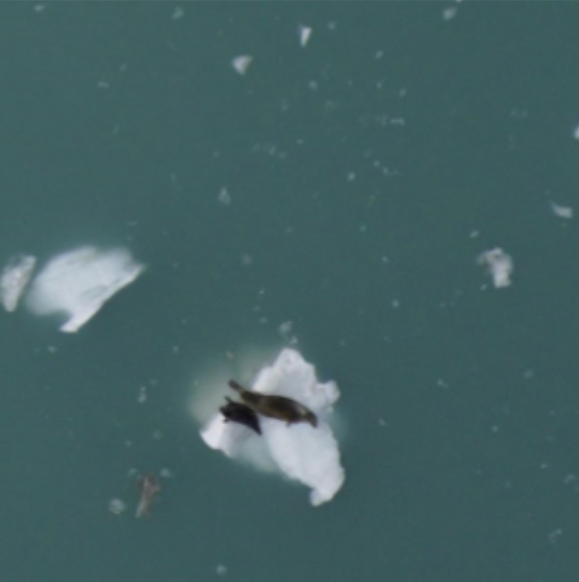
Aerial wildlife camera photo of a seal hauled out on an ice floe

Click any cell to move the 2×2 occlusion patch · gray block = baseline fill

Score-drop map — darker red means covering that patch hurt P(seal) more

Original P(seal)

0.880

Occluded P(seal)

0.460

Score drop

0.420

Patch (row 3, col 2) covers the seal's head.

Occlusion gives direct behavioral evidence, but patch size and replacement color determine what is removed and how artificial the input becomes.

Occlusion is easy to explain and model agnostic. It can also create inputs the model has never seen. A gray square over an X-ray is an artifact, and deleting one word can break grammar. Choose a replacement that makes sense for the domain and vary patch size so the explanation does not depend on one arbitrary mask.

Photorealistic inpainting perturbations for occlusion-based explanations

NeurIPS Imageomics Workshop 2025

Photorealistic Inpainting for Perturbation-based Explanations in Ecological Monitoring

Instead of masking or blurring regions, this method uses inpainting to generate photorealistic, in-distribution edits -- swapping or removing subjects while preserving scene context -- to produce more reliable occlusion-based explanations for vision models.

Aghakishiyeva et al. (an XAI alum!)Read the Paper

Checkpoint

Why might a large occlusion patch overestimate a region's importance?

←PreviousLayer-Wise Relevance PropagationAttribution-Based Explanations Next→Concept Activation Vectors (TCAV)Concept-Based Explanations