Methods
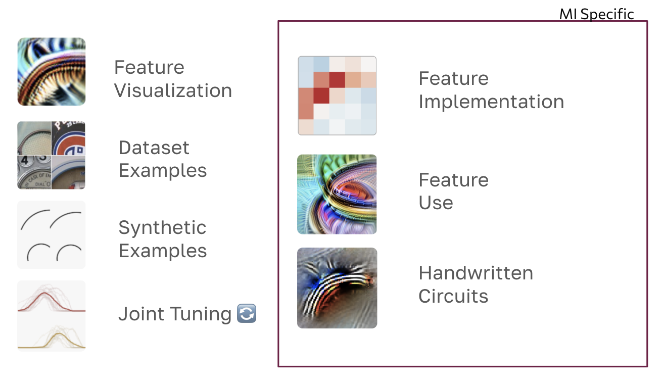
How do researchers actually investigate a candidate feature? Mechanistic interpretability draws on a handful of recurring methods. Some are general-purpose techniques borrowed from XAI; others are MI-specific — developed for the purpose of reverse-engineering a network's internals.
Method families
- Perturbation-based methods: ablation, activation patching, causal tracing, path patching, and causal scrubbing.
- Output attribution: logit difference, per-token loss, direct logit attribution, and logit lens.
- Scoring and probing: scores such as induction or compositionality measures that summarize model behavior.
- Visualization and interpretation: feature visualization and max-activating dataset examples.
- Representation learning: dictionary learning and sparse autoencoders.
- Architectural modifications: changes such as linearizing LayerNorm to make internal structure easier to analyze.

Feature visualization optimizes an input from scratch to make a chosen component fire as strongly as possible. Because every pixel in the resulting image was added by the optimization process in order to cause the neuron to fire, the result reflects what the component is sensitive to, rather than what happens to appear in any one photograph.
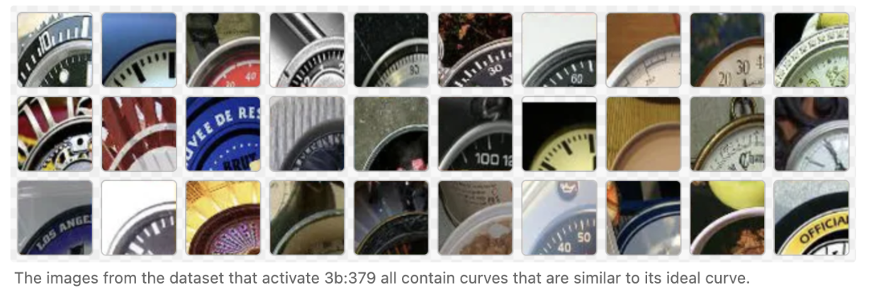
Dataset examples take the opposite approach: instead of generating an input, search a real dataset for the examples that activate a component most strongly. This shows what actually activates the component under naturalistic conditions, which can differ from what an unconstrained optimizer finds.
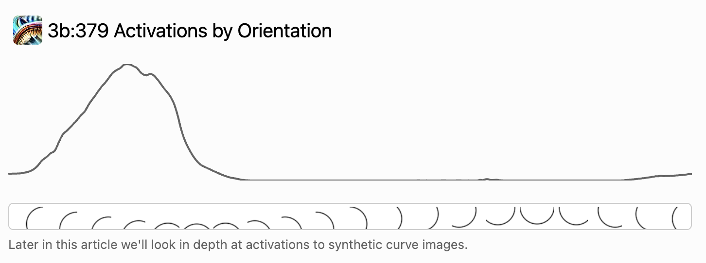
Synthetic examples replace natural images with stimuli the researcher builds by hand, varying one property at a time — orientation, curvature, color, scale. Because the experimenter controls every property of the input, this method can isolate a specific variable in a way that natural dataset examples usually cannot.
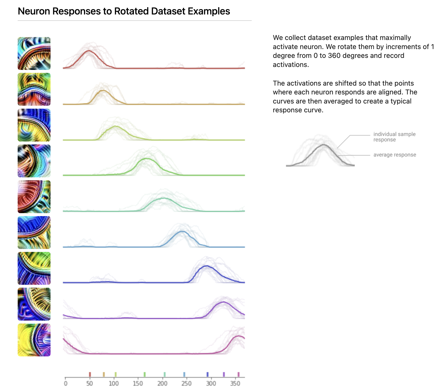
Joint tuning varies a stimulus continuously, such as rotating a shape through all orientations, while tracking several related components at once. This reveals how components in a family divide up a continuous variable between them, rather than characterizing any single component in isolation.
MI-specific methods
Feature visualization, dataset examples, synthetic examples, and joint tuning are behavioral: they characterize a component from its input-output responses without opening it up. The next three methods look inside the network itself.
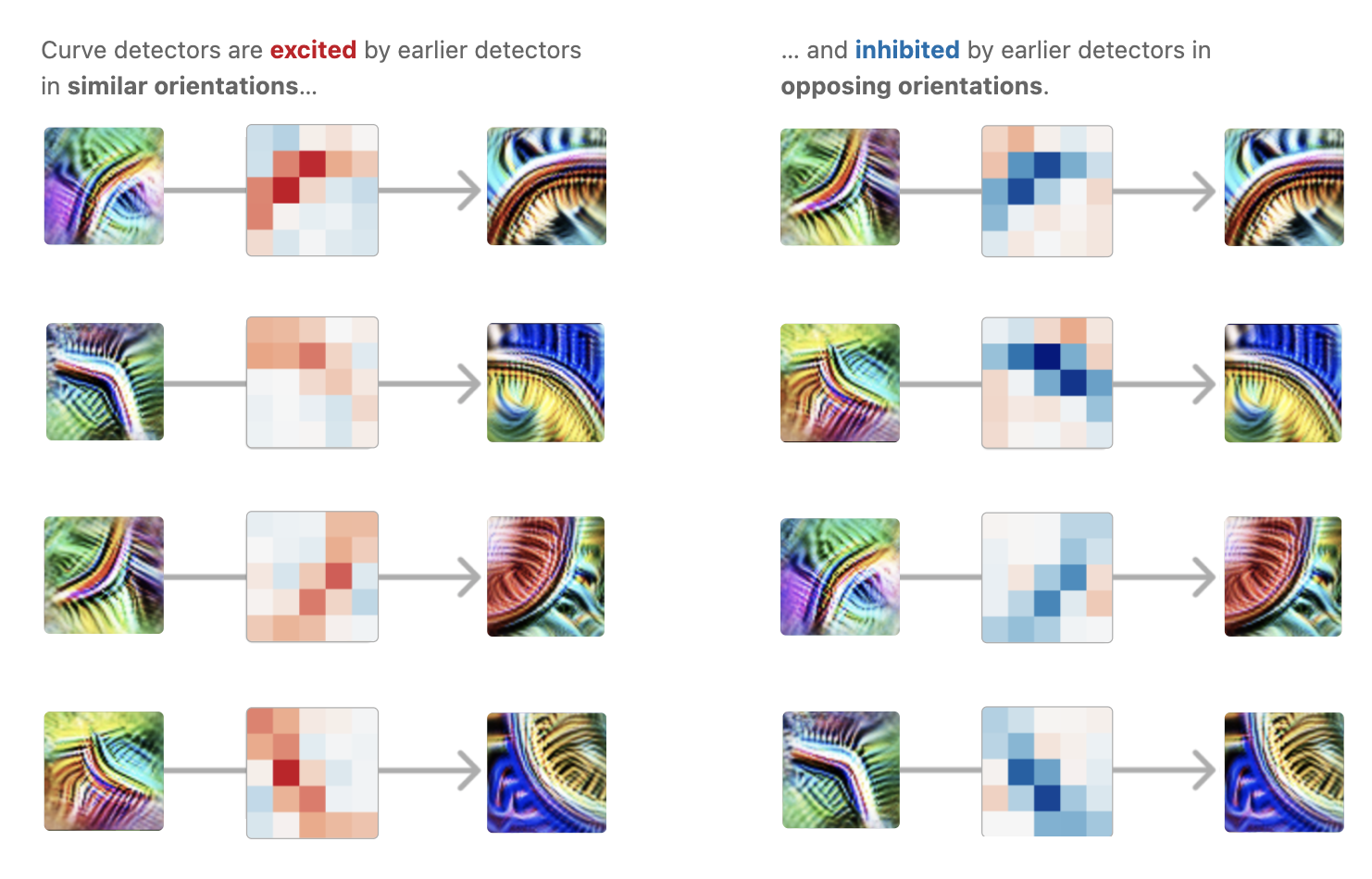
Feature implementation inspects the circuit that constructs a component — the signed weights connecting it to earlier components. Reading those weights can reveal the algorithm a component computes from its inputs, rather than only describing what the component responds to from the outside.
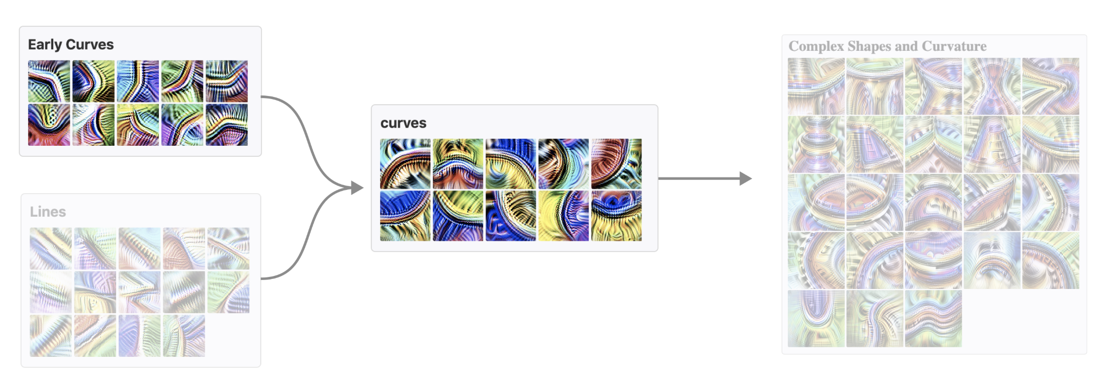
Feature use looks the other direction: at the downstream components that read from a given component. Inspecting how those clients weight and combine the component's output can reveal what role the component plays in the larger computation, beyond what it responds to.
Handwritten circuits go a step further than inspecting weights: a researcher hand-sets every weight in a small circuit to implement a hypothesized algorithm from scratch, with no learned parameters. If the handwritten circuit reproduces the behavior of the trained network, the hypothesized algorithm is at least sufficient to explain it.
Build a Curve-Detection Circuit
Change the early edge detectors and step through the computation. Excitatory weights add compatible evidence; an inhibitory weight subtracts an opposing orientation.
1. Input evidence
left edge
0.85
right edge
0.75
opposing
0.20
curve
0.90
circle client
0.97
Adjust the early edge detectors and step through implementation and use: weighted edges build the curve feature, which a downstream circle client then reads.
A researcher wants to know how a component's output is actually used by the rest of the network, not just what makes the component fire. Which method addresses that question, and why don't feature visualization or dataset examples answer it?